Write Buffering, LSM Tree, & Journaling Summarized

13 Jun 2020 - Guanzhou Hu

Back to List of Blogs

In file system & database design, write buffering (write grouping or coalescing) is a commonly-used technology to avoid in-place updates and only expose sequential writes to disks. Log-Structured Merge Tree (LSM tree) is a modern practical solution which sacrifices a little bit of read performance to enable efficient write buffering. Journaling (write-ahead logging) is another file system terminology which is sometimes confused with write buffering. In short, write buffering is for write performance and journaling is for crash recovery - they are different, but can be combined.

(I previously misused the terminology of write-ahead logging and confused it with write buffering. This is now a newer version of the post.)

Background

In file systems and databases where files/records are allowed to grow, a file made up of multiple contiguous logical blocks may actually consist of multiple noncontiguous physical blocks on disk. Thus, a mapping from a logical block number to a physical block is at the essence.

\[f: \text{logical# } l \in \mathbb{Z} \mapsto \text{physical block } p.\]

We can implement such a mapping in different ways. For example:

• Each physical block stores its corresponding logical# \(l\), together with pointers to the two physical blocks of adjacent logical blocks \(l-1\) and \(l+1\). We have to start with some physical block \(p\) and traverse through the path, involving many IOs. (Used in old navigational databases.)
• Separate the logical navigation structure apart from physical data, attaching physical# \(p\) as satellite value to keys \(l\). Search the logical navigation structure for logical number \(l\) to get the pointer \(p\). (This is called an ISAM design¹.) A navigation structure can take many different forms:
  • Simple linked-list
  • Hash table
  • Balanced binary search tree: Red-black tree, AVL tree
  • B tree / B+ tree
  • …

Notice that the navigation structure itself is also stored in persistent storage. This is partly because the structure itself is quite big. Also, we have to accommodate memory crash failures. A UNIX-flavor file system, such as Ext4, often use a B+ tree² as part of a file’s metadata (called an inode structure). The following figure demonstrates a simplified disk content layout of such file systems.

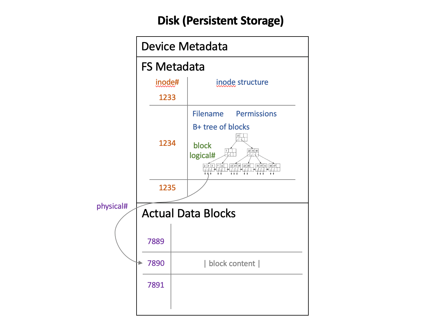
The downside of using a navigation structure is that writes perform badly. Disks are way better at sequential appends than at random in-place updates, especially on HDDs. To write to a file, we always have to go back to the structure and update the structure. Worse, if the write itself is an update to file content, we end up with two in-place updates. To optimize for write-heavy workloads, people use write buffering.

Write Buffering Solutions

This section is based on Ben’s blog post³. The essential motivation of write buffering is to transform write operations into pure sequential appends. We call a logical# as a key and its corresponding block content as its value. (This model also naturally fits in a key-value database.) The disk purely stores a monotonically growing log whose entries are new key-value pairs.

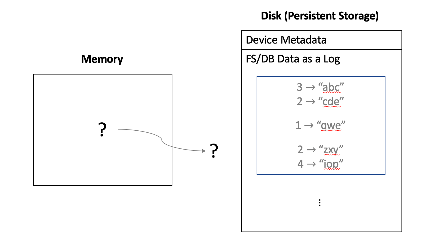
How to manage this log then?

Solution 1: Maintain an in-memory hash map from key to log entry of its latest value. This is impractical since this hash map can be very large and probably cannot fit in memory.

Solution 2: Build the entire log as an append-only B tree⁴ (READ HERE). The problem is that append-only B trees have significant write-amplification problems, thus not very attractive.

Solution 3: Use a Log-Structured Merge Tree (LSM Tree)⁵. This sacrifices a little bit of read performance.

LSM Tree & Details

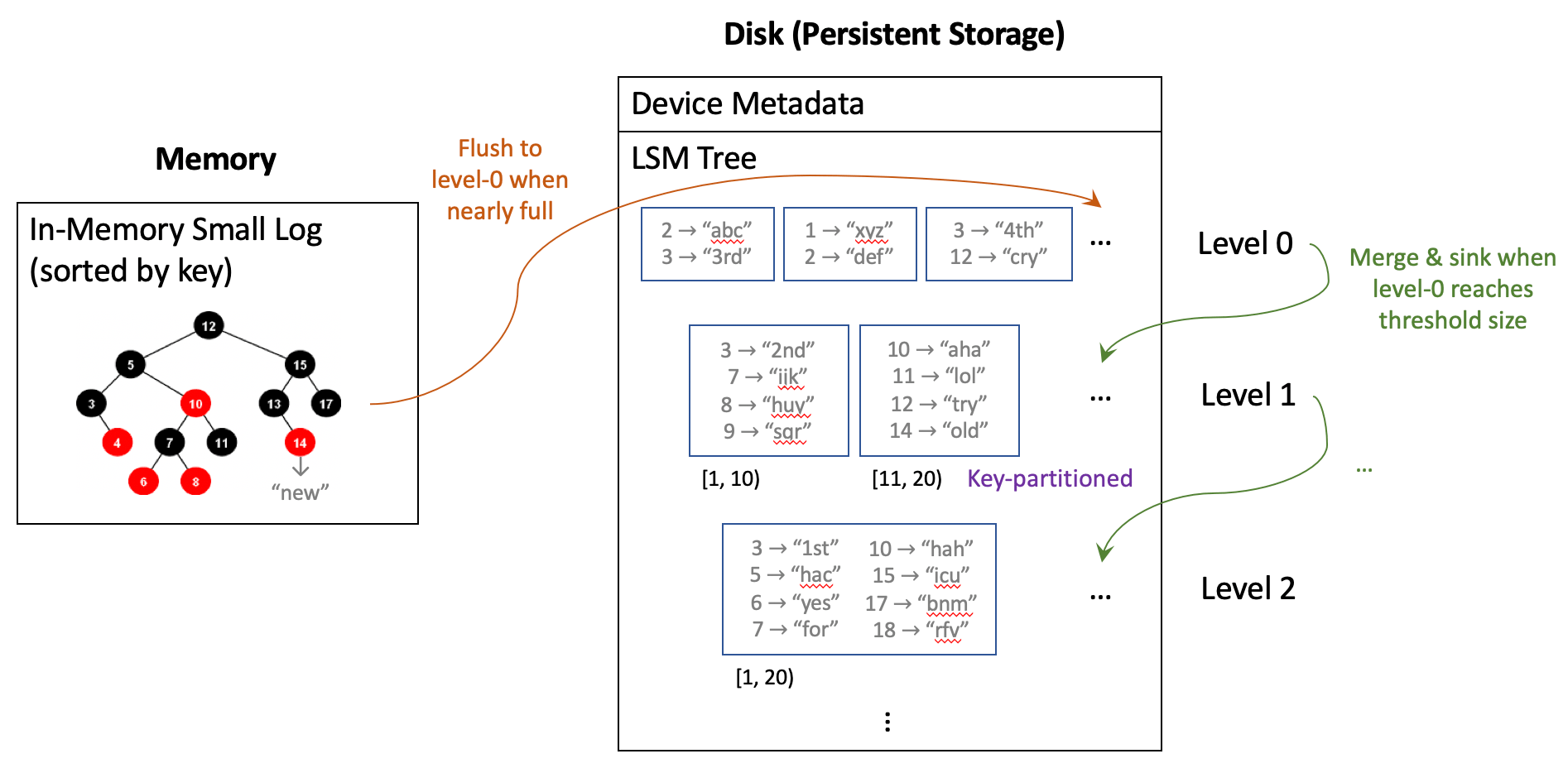
An LSM tree requires coordination between an in-memory small sorted log and persisted data log on disk. We reserve space for a small sorted data structure, e.g., a red-black tree, in memory. As new writes come, we insert the new key-value pair into this red-black tree, sorted by keys. When this small in-memory log becomes nearly full, a flush is triggered to persist this sorted batch to disk. The on-disk log is called the level-0 log and is monotonically growing. This is the “log-structured” part of an LSM tree.

Well, if an LSM tree is only this simple, you can easily notice the problem here - reading out value of a key \(l\) is very inefficient. If \(l\) is not in the in-memory red-black tree at the time of read, we have to traverse the disk log in reverse chronological order, find the first batch containing \(l\), and then read out the value of \(l\) in that batch. This is unacceptable and we must restrict the total number of batches.

So here we introduce the “merge” part of an LSM tree. From time to time, we merge the level-0 log batches into a whole big batch, remove duplicate old keys, and sink it down one level below. Since each small batch is inherently sorted, such a merge can be done efficiently. By periodically merging, we restrict the number of level-0 batches to a threshold of \(t\) batches. We can so the same thing for level-1 and build a multi-level LSM tree.

We call this operation merge, sink, compact, or compress. They all mean the same thing.

We further introduce two additional optimizations to boost read performance and robustness. First, starting from level-1, keys are partitioned across batches and each batch holds a distinct range of keys. This makes merge operations not “very sequential” but searching for a key in level-1 or higher only touches one batch. Second, checking whether a batch contains a key can be boosted by using a bloom filter⁶.

The following figure demonstrates memory and disk content layout of an LSM tree.

Reading the value of a key \(l\) follows three steps:

1. Check if \(l\) exists in the in-memory red-black tree. If so, return its value; Else, continue to step 2.
2. In reverse order, traverse through on-disk level-0 batches and search for key \(l\). Once found, return its value; If no batches hold \(l\), continue to step 3.
3. Starting from level-1, check the batch whose range covers \(l\). If found, return its value; Else, go one level deeper and repeat step 3.

Say we restrict number of level-0 batches to \(t\) and the maximum depth is level-\(d\). Define the approximate time taken to search for a key in a sorted batch as \(1\) unit (ignore size differences among batches). Reading a value from an LSM tree takes at most \(1 + t + d\).

Multiple versions of a key can exist in the log at the same time, where the newest version resides in the “highest” level. In practical systems, we must also pay attention to garbage collection to clear out obselete versions.

Systems that adopt LSM tree design include Google Bigtable, LevelDB, RocksDB, Cassandra, InfluxDB, and many more.

Journaling (Write-Ahead Logging)

Another confusing term also used in file systems is journaling, or write-ahead logging. Journaling describes an advanced way of “flushing things from memory to disk” to support fast crash recovery⁷. Originally, if the system crashes in the middle of a read/write/delete operation and later restarts, data on persistent storage might be partial and inconsistent. This inconsistency can only be recovered through a complete checksum walk over the whole file system (a file system check, fsck).

A journaling file system keeps a journal on disk (should call it journal here to avoid confusion with the log in write buffering). It logs an operation into the journal, commits this logging, and only then acks the user and applies this operation. After crashing, it simply replays committed operations in the journal to recover and ignores all uncommited entries. The downside is that every write must be carried out twice, called write-twice penalty.

For a weaker consistency model, some journaling file systems perform in a so-called ordered mode, which just journals metadata updates but not updates to data blocks. Data block allocation and writes happen first, followed by metadata journal append. In this mode, operations like append are crash-consistent, but in-place write updates are vulnerable to crashes.

For a file system which uses write buffering, it is natural to think that, since the actual data itself is a log (or something like a log, e.g., an LSM tree), why don’t we just use this as the journal? A file system which combines write buffering and journaling in this way is called a log-structured file system (LFS)^{8 9}. The log itself is the FS. It benefits from both sequential writes and faster crash recovery, without write-twice penalty. However, every update (to either metadata or data) must be appended as a new entry to the log, invalidating some old entries. The system must then deploy some sort of garbage collection mechanism to clean up the log periodically, discarding invalid log entries and compacting valid entries.

Examples of non-log-structured journaling file systems include Linux Ext3 and Ext4. Examples of log-structured file systems include LFS, WAFL, ZFS, Btrfs, and NOVA.

References

1. https://en.wikipedia.org/wiki/ISAM ↩

2. https://en.wikipedia.org/wiki/B%2B_tree ↩

3. http://www.benstopford.com/2015/02/14/log-structured-merge-trees/ ↩

4. http://www.bzero.se/ldapd/btree.html ↩

5. https://en.wikipedia.org/wiki/Log-structured_merge-tree ↩

6. https://en.wikipedia.org/wiki/Bloom_filter ↩

7. https://en.wikipedia.org/wiki/Journaling_file_system ↩

8. http://pages.cs.wisc.edu/~remzi/OSTEP/file-lfs.pdf ↩

9. https://people.eecs.berkeley.edu/~brewer/cs262/LFS.pdf ↩

Back to List of Blogs

Please comment below anything you wanna say! 😉

Back to Top