Linearizability

With multiple nodes issuing and completing concurrent operations on a single object, linearizability ^{1 2} is defined as the conjunction of the following two conditions:

• there must exist an equivalent global sequential order of all operations, where each operation observes the results of all preceding operations, and
• the global order must obey the real-time property: if an operation starts later than another one finishes (based on their timestamps), it must be placed after that one in the global order.

The core idea behind this algorithm is to maintain a set of still-possible states (hereafter called possibilities) given the operation results observed. If this set ever becomes empty after feeding an operation result in, then linearizability has been violated.

Definitions

Each possibility is a “snapshot” of the object’s value after successfully applying a sequence of operations. More precisely, a possibility tracks the following three things:

• lineage history: the sequence of operations that have been applied; think of this as the determined prefix of a possible global sequential order
• current value: the current value of the object, obtained by starting from an initial nil value and applying the determined sequence
• per-node queues: per-node queues of operation results coming from each node which have not been applied yet

where each operation result, denoted <ts_req>Type(in/out)<ts_ack>, contains the following information besides its source node ID:

• ts_req: starting timestamp
• Type(in/out): Put input/Get output
• ts_ack: finish timestamp

Let’s assume all timestamps are unique, and operations from each node are always already in order (i.e., ts_req of the next operation fed by a node is always > ts_ack of its previous operation).

Here is an example of a valid possibility, assuming a known number of 2 nodes n0 and n1:

The Algorithm

The checker starts from an initial set that contains only one initial possibility.

Nodes feed completed operations to the checker. For each operation fed, the checker pushes it to the back of the corresponding node’s queue of every current possibility. Say node n0 feeds a Put(55) that started on timestamp 1 and finished on 5:

The checker tries to step each current possibility by consuming it, producing 0-to-some new possibilities, and adding them to the set. A possibility can be stepped iff. it has at least one pending operation from every node. Here, there’s now only one possibility in the set and it cannot be stepped (as we don’t yet know what the next op from n1 would look like), so nothing happens.

Say n1 then feeds a Put(66):

Now we know at least one operation from every node for this possibility, meaning it can be stepped. It picks candidate operations from heads of per-node queues and tries to apply the op to its current value; a successful apply produces a new possibility, while a Get with mismatching value produces none. In this case, either head is a valid candidate because their timestamp spans overlap and both are just Puts. After stepping, the possibility is consumed and two new valid possibilities are produced, so the set now looks like:

Stepping is attempted repeatedly until all possibilities in the new set cannot be stepped.

Say n1 then feeds a Get(77) that started late:

While this may look like a linearizability violation at first glance, we can’t say for sure because n0 could have made a Put(77) sometime in the middle. Anyways, feeding this Get makes the second possibility steppable; but this time, only the Put(55) can be a valid next operation. The Get(77) cannot be chosen as a candidate because of two reasons: 1. it started strictly after the finish of Put(55), and 2. even if it overlapped with the Put, its output does not match the current value 66. The new set after stepping:

Say n0 then feeds a Put(77) which indeed happened in the middle:

After stepping all current possibilities exhaustively, the set reduces to one possibility, and linearizability still holds.

Note that operations Put(66) and Put(55) are swappable in the lineage history, but we consider both as the same possibility as they don’t affect the checker’s decisions beyond.

Consider, alternatively, that n0 instead feeds an arbitrary operation that started at timestamp 13, rather than a Put(77) that started before 12. You should find no valid possibilities left after exhaustive stepping, meaning a linearizability violation is detected: n1’s Get that finished at timestamp 12 cannot observe a value of 77. I will leave this as an exercise for readers =)

Implementation

An implementation of this algorithm, along with examples, can be found at this GitHub repo ³.

References

Files of This TLA+ Spec

Below are the files composing the checkable model (organized in VSCode extension style):

• MultiPaxos.tla (main protocol spec written in PlusCal and with translation attached)
• MultiPaxos_MC.tla (entrance of running model checking; contains the checked constraints)
• MultiPaxos_MC.cfg (recommended model inputs and configurations, which should give 100% coverage of all interesting cases)
• MultiPaxos_MC_small.cfg (smaller input with one fewer write and no CommitNotice messages)

What’s Good About This Spec

This spec is different from traditional, general descriptions of Paxos/MultiPaxos in the following aspects:

• It models MultiPaxos in a practical SMR system style that’s much closer to real implementations than its traditional, abstract specs (e.g., this)
  • All servers explicitly replicate a log of instances, each holding a command
  • Numbers of client write/read commands are made model inputs
  • Explicit termination condition is defined, thus semi-liveness can be checked by not having deadlocks
  • Safety constraint is defined as a clean client-viewed linearizability property upon termination
  • Replica node failure is injected to assure the protocol’s fault-tolerance level
  • See the detailed comments in the source files…
• Careful optimizations are applied to the spec to reduce the state space W.L.O.G.
  • Model checking with recommended inputs completes in < 22 min on a 40-core server machine
  • Commenting out the HandleCommitNotice action (which is the least significant) and having one fewer request reduces check time down to < 10 secs
• It is easy to extend this spec and add even more practical features
  • Leader lease and local read
  • Asymmetric write/read quorum sizes
  • …

This spec has been accepted into the official TLA+ Examples repo! ¹

Here are some links I found particularly useful when developing this spec by myself: ^{2 3 4 5}

Update: Extended Spec with Extra Features

Below are the files composing an extended version of the spec along with model inputs:

• MultiPaxos.tla (extended main protocol spec written in PlusCal and with translation attached)
• MultiPaxos_MC.tla (entrance of running model checking; contains the checked constraints)
• MultiPaxos_MC.cfg (recommended model inputs and configurations, which should give 100% coverage of all interesting cases with default features)
• MultiPaxos_MC_small.cfg (smallest input for sanity check)
• MultiPaxos_MC_rwqrm.cfg (input demonstrating asymmetric write/read quorum sizes)
• MultiPaxos_MC_lease.cfg (input demonstrating stable leader leases and local read)

What’s New in the Extended Spec

The extended spec includes the following extra features/variants of MultiPaxos that are very essential and useful in practice:

• Only keep writes in the log (while reads squeeze in between writes)
• Asymmetric write/read quorum sizes
• Stable leader lease and local read at leader

References

This post assumes latest Linux kernel version and is tested on v6.5.7.

Problem Setting

I have a distributed system codebase consisting of the following processes, each of which should conceptually run on a separate physical machine:

• \(S\) server nodes,
• \(C\) client nodes,
• and one manager node.

W.L.O.G., let’s ignore the client nodes and only talk about the server nodes plus the manager. I would like to test a wide range of different network performance parameters on the network connections between servers. Doing that across real physical machines would be prohibitively resource-demanding (as it requires a bunch of powerful machines all connected with each other through physically links that are as strong as the “best parameters” you will test against). Processes in my codebase are not computation- or memory-demanding, though; so it might be a good idea to run them on a single host and emulate a network environment among them.

There’re not really any canonical tutorials online demonstrating how to do this. After a bit of searching & digging, I found Linux kernel-supported network emulation features to be quite promising.

First Try: tc netem on LoopBack

The first tool to introduce here is the netem queueing discipline (qdisc) ¹ provided by the tc traffic control command. Each network interface in Linux can have an associated software queueing discipline that sits atop the device driver queue. netem is one of them and it provides functionality for emulating various network properties, including delay, jitter distribution, rate, loss, corruption, duplication, and reordering, etc.

For example, we can put a netem qdisc on the loopback interface that injects a 100ms delay with a Pareto-distributed jitter around 10ms and limits the rate as 1Gbps:

~$ sudo tc qdisc add dev lo root netem delay 100ms 10ms distribution pareto rate 1gibit
~$ ping localhost
PING localhost (127.0.0.1) 56(84) bytes of data.
64 bytes from localhost (127.0.0.1): icmp_seq=2 ttl=64 time=192 ms
64 bytes from localhost (127.0.0.1): icmp_seq=4 ttl=64 time=226 ms
64 bytes from localhost (127.0.0.1): icmp_seq=5 ttl=64 time=193 ms
...

It feels natural to just put a netem qdisc on the loopback interface, let all processes bind to a different port on localhost, and let them talk to each other all through loopback. It seemed to work pretty well until I found two significant caveats:

1. Since all process transfer packets through the same loopback interface, packets with different source-destination pairs will all be congesting with each other in the same queue, creating unwanted interference and often overflowing the loopback queue.
2. Only one netem qdisc is allowed on each interface. This means we cannot emulate different parameters for different links among different pairs of processes.

What we need are separate network interfaces for the processes.

Didn’t Work: dummy Interfaces

The dummy kernel module supports creating dummy network interfaces that route packets to the host itself. However, creating a netem qdisc on a dummy interface doesn’t really work ^{2 3}.

~$ sudo ip link add dummy0 type dummy
~$ sudo ip addr add 192.168.77.0/24 dev dummy0
~$ sudo ip link set dummy0 up
~$ sudo tc qdisc add dev dummy0 root netem delay 10ms
~$ sudo tc qdisc show
...
qdisc netem 80f8: dev dummy0 root refcnt 2 limit 1000 delay 10ms

Though the qdisc is indeed listed, pinging the associated address still shows lightning-fast delay:

~$ ping 192.168.77.0
PING 192.168.77.0 (192.168.77.0) 56(84) bytes of data.
64 bytes from 192.168.77.0: icmp_seq=1 ttl=64 time=0.019 ms
64 bytes from 192.168.77.0: icmp_seq=2 ttl=64 time=0.024 ms
64 bytes from 192.168.77.0: icmp_seq=3 ttl=64 time=0.024 ms
...

This is because the dummy interface is just a “wrapper”; it is still supported by the loopback interface behind the scene. We can verify this fact using:

~$ sudo ip route get 192.168.77.0
local 192.168.77.0 dev lo src 192.168.77.0 uid 0
    cache <local>

Notice it is reported that the route is backed by dev lo. In fact, if a netem qdisc is still being applied to loopback as of previous section, you will see that delay when pinging dummy0. Dummy is not we are looking for here.

Solution: Network Namespaces & veths

What we are actually looking for are network namespaces and veth-type interfaces ^{4 5}. In Linux, a network namespace is an isolated network stack that processes can attach to. By default, all devices are in a nameless namespace. One can create named namespaces using ip netns commands and assign them to running processes (or launch new processes directly from them through ip netns exec). Namespaces are a perfectly tool for our task here.

To give connectivity between namespaces without bringing in physical devices, one can create veth (virtual Ethernet) interfaces. By design, veth interfaces come as pairs: you must create pairs of two veths at the same time. This post ⁶ gives a nice demonstration of creating two namespaces and making a pair of veths to connect them.

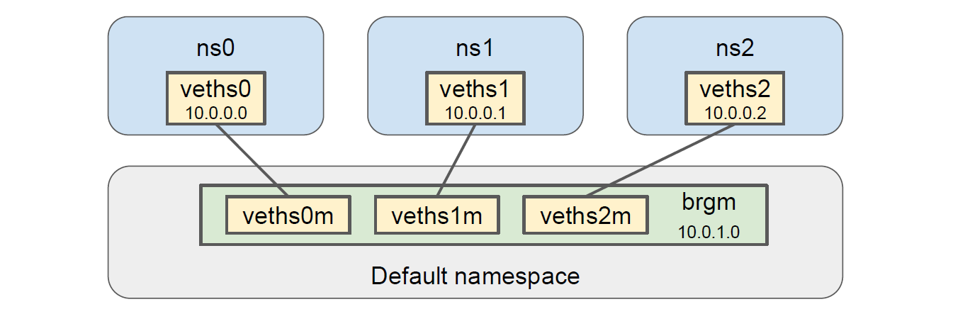
However, this is not enough for us, because we would want more than 2 isolated devices, each being able to talk to everyone else. To achieve this, we make use of a bridge device. We create one pair of veths per namespace, put one end into the namespace while keeping the other end, and then bridge those ends together. All namespaces can then find a route to each other through the bridge; also, the bridge can talk to each of the namespaces. Since we have a manager process, it is quite natural to let the manager use the bridge device and let each server process reside in its own namespace and use the veth device put into it.

Let’s walk through this step-by-step for a 3-servers setting.

1. Create namespaces and assign them proper IDs:

    ~$ sudo ip netns add ns0
    ~$ sudo ip netns set ns0 0
    ~$ sudo ip netns add ns1
    ~$ sudo ip netns set ns1 1
    ~$ sudo ip netns add ns2
    ~$ sudo ip netns set ns2 2
   

2. Create a bridge device brgm and assign address 10.0.1.0 to it:

    ~$ sudo ip link add brgm type bridge
    ~$ sudo ip addr add "10.0.1.0/16" dev brgm
    ~$ sudo ip link set brgm up
   

3. Create veth pairs (vethsX-vethsXm) for servers, put the vethsX end into its corresponding namespace, and assign address 10.0.0.X to it:

    ~$ sudo ip link add veths0 type veth peer name veths0m
    ~$ sudo ip link set veths0 netns ns0
    ~$ sudo ip netns exec ns0 ip addr add "10.0.0.0/16" dev veths0
    ~$ sudo ip netns exec ns0 ip link set veths0 up
    # repeat for servers 1 and 2
   

4. Put the vethsXm end under the bridge device:

    ~$ sudo ip link set veths0m up
    ~$ sudo ip link set veths0m master brgm
    # repeat for servers 1 and 2
   

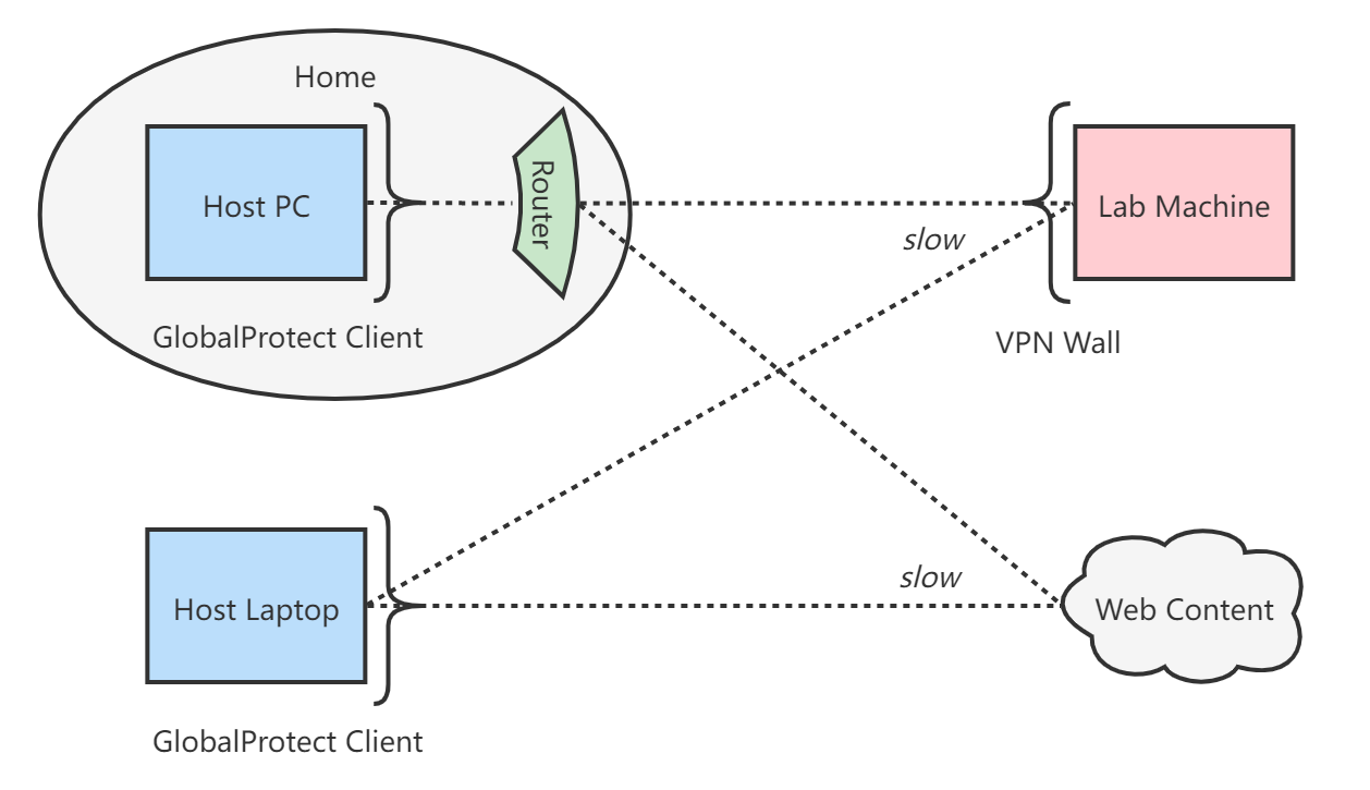
This gives us a topology that looks like the following figure:

Let’s do a bit of delay injection with netem to verify that this topology truly gives us what we want. Say we add 10ms delay to veths1 and 20ms delay to veths2:

~$ sudo ip netns exec ns1 tc qdisc add dev veths1 root netem delay 10ms
~$ sudo ip netns exec ns2 tc qdisc add dev veths2 root netem delay 20ms

Pinging the manager from server 1:

~$ sudo ip netns exec ns1 ping 10.0.1.0
PING 10.0.1.0 (10.0.1.0) 56(84) bytes of data.
64 bytes from 10.0.1.0: icmp_seq=1 ttl=64 time=10.1 ms
64 bytes from 10.0.1.0: icmp_seq=2 ttl=64 time=10.1 ms
64 bytes from 10.0.1.0: icmp_seq=3 ttl=64 time=10.1 ms
...

Pinging server 2 from server 1:

~$ sudo ip netns exec ns1 ping 10.0.0.2
PING 10.0.0.2 (10.0.0.2) 56(84) bytes of data.
64 bytes from 10.0.0.2: icmp_seq=1 ttl=64 time=30.1 ms
64 bytes from 10.0.0.2: icmp_seq=2 ttl=64 time=30.1 ms
64 bytes from 10.0.0.2: icmp_seq=3 ttl=64 time=30.1 ms
...

All good!

There are also obvious ways to extend this topology to allow even more flexibility; for example, each server’s could own multiple devices in its namespace that have different connectivity and different performance parameters, etc. Let me describe one example extension below.

Extension: Symmetric Ingress Emulation w/ ifbs

It is important to note that most of netem’s emulation functionality applies only to the egress side of the interface. This means all the injected delay happen on the sender side for every packet. In some cases, you might want to put custom performance emulation on the ingress side of the servers’ interfaces as well. To do so, we could utilize the special IFB devices ⁷.

First, load the kernel module that implements IFB devices:

~$ sudo modprobe ifb

By default, two devices ifb0 and ifb1 are added automatically. You can add more by doing:

~$ sudo ip link add ifb2 type ifb

We then bring one IFB device to each server’s namespace and redirect all the incoming traffic to the veth interface to go through the ifb device’s egress queue first. This is done by adding a special ingress qdisc to the veth (which can exist simultaneously with an egress netem qdisc we added earlier) and placing a filter rule to simply “move” all ingress packets to the ifb interface’s egress queue. The ifb device will automatically move the packet back after it has gone through the ifb’s egress queue.

~$ sudo ip link set ifb0 netns ns0
~$ sudo ip netns exec ns0 tc qdisc add dev veths0 ingress
~$ sudo ip netns exec ns0 tc filter add dev veths0 parent ffff: protocol all u32 match u32 0 0 flowid 1:1 action mirred egress redirect dev ifb0
~$ sudo ip netns exec ns0 ip link set ifb0 up

We can then put a netem qdisc on the ifb interface, which effectively emulates specified performance on the ingress of the veth. For example:

~$ sudo ip netns exec ns0 tc qdisc add dev ifb0 root netem delay 5ms rate 1gibit

Summary

To achieve our goal of emulating network links among distributed processes, on a single host, beyond the limitation of a single loopback interface, we can take the following steps:

• Create separate network namespaces, probably one for each process, using ip netns.
• Create veth interface pairs, probably one pair for each process, using ip link ... type veth.
• Put one end of each veth pair into the corresponding namespace, then keep the other ends and create a bridge that stitches them together.
• Use tc qdisc ... netem to apply the netem queueing discipline with desired parameters on the veth devices for each process.
• Run the processes with their corresponding network namespace attached.

Below is a script for setting up the above described topology for a given number of server processes:

#! /bin/bash

NUM_SERVERS=$1


echo
echo "Deleting existing namespaces & veths..."
sudo ip -all netns delete
sudo ip link delete brgm
for v in $(ip a | grep veth | cut -d' ' -f 2 | rev | cut -c2- | rev | cut -d '@' -f 1)      
do
    sudo ip link delete $v
done


echo
echo "Adding namespaces for servers..."
for (( s = 0; s < $NUM_SERVERS; s++ ))
do
    sudo ip netns add ns$s
    sudo ip netns set ns$s $s
done


echo
echo "Loading ifb module & creating ifb devices..."
sudo rmmod ifb
sudo modprobe ifb  # by default, add ifb0 & ifb1 automatically
for (( s = 2; s < $NUM_SERVERS; s++ ))
do
    sudo ip link add ifb$s type ifb
done


echo
echo "Creating bridge device for manager..."
sudo ip link add brgm type bridge
sudo ip addr add "10.0.1.0/16" dev brgm
sudo ip link set brgm up


echo
echo "Creating & assigning veths for servers..."
for (( s = 0; s < $NUM_SERVERS; s++ ))
do
    sudo ip link add veths$s type veth peer name veths${s}m
    sudo ip link set veths${s}m up
    sudo ip link set veths${s}m master brgm
    sudo ip link set veths$s netns ns$s
    sudo ip netns exec ns$s ip addr add "10.0.0.$s/16" dev veths$s
    sudo ip netns exec ns$s ip link set veths$s up
done


echo
echo "Redirecting veth ingress to ifb..."
for (( s = 0; s < $NUM_SERVERS; s++ ))
do
    sudo ip link set ifb$s netns ns$s
    sudo ip netns exec ns$s tc qdisc add dev veths$s ingress
    sudo ip netns exec ns$s tc filter add dev veths$s parent ffff: protocol all u32 match u32 0 0 flowid 1:1 action mirred egress redirect dev ifb$s
    sudo ip netns exec ns$s ip link set ifb$s up
done


echo
echo "Listing devices in default namespace:"
sudo ip link show


echo
echo "Listing all named namespaces:"
sudo ip netns list


for (( s = 0; s < $NUM_SERVERS; s++ ))
do
    echo
    echo "Listing devices in namespace ns$s:"
    sudo ip netns exec ns$s ip link show
done

References

Revisited Material

• Decentralized Thoughts blog series: a really good blog series on consensus problems. Although most of the advanced blog posts there focus on decentralized Byzantine-fault-tolerant systems, the beginner posts offer a great summary of the problem and the foundational models we are studying.
• My practical technical report: a “somewhat formal” summary of non-transactional consistency models and availability models for distributed replication. This report corrects some inaccuracy/errors in my previous blog post and extends it to a broader scope.

Traditional Locking

Consider a database with only one small table (i.e. relation), shared by multiple clients. The clients could issue concurrent transactions that read some tuples (i.e. records) of the table or update them with new values. To protect the database from data races, it is pretty natural to apply a traditional reader-writer lock on the table.

In database terminology, we denote acquiring a reader lock on the table as locking it in shared (S) mode, while acquiring a writer lock on the table as locking it in exclusive (X) mode. Multiple clients could hold S locks on the same table at the same time for reads. At most one client could hold an X lock on the table (with no S locks held by anyone else as well).

We call two locking attempts compatible if their lock modes are allowed to be held at the same time on the same thing. S mode is compatible with itself. S and X are not compatible with each other. X is of course also not compatible with itself.

Back to our problem scenario, since the database has only one table with a small number of tuples, a reasonable solution is to put a lock on that table. Read requests must attempt to acquire the lock in S mode and can proceed only after the acquirement is successful. Writes requests must attempt to acquire it in X mode. This is basically how a reader-writer lock works in classic systems. So far, so good.

Problem: what if the database is not in toy scale any more, but is composed of hundreds of tables, each having millions of records? Real-world databases can easily reach this scale. The traditional locking mechanism with uniform granularity puts a dilemma on choosing the granularity of locks:

• Huge DB lock: we could choose to lock on coarse granularity, e.g., the entire database. However, it unacceptably hurts concurrency; a client transaction updating only one tuple in one table would block all other clients that try to read disjoint sets of tuples in the database.

• One lock per tuple: alternatively, we could choose to put locks only at the finest granularity, in this case, tuples. A client transaction only locks the tuples it would touch in desired mode. This way, concurrency is preserved. The problem is that it forces large transactions to touch too many locks; e.g, a transaction that scans all tuples of a table will have to acquire potentially millions of locks. This can easily lead to prohibitive performance overhead.

Both choices are not ideal for overall performance. The solution to this problem is to introduce hierarchical locking on different levels of database resources.

Hierarchical Locking

A database is naturally structured as a tree (or more generally, a DAG) of resources. For example, the following figure represents a database with 3 tables, each having 100 tuples. Tuples could further be decomposed into fields (i.e. attributes or columns); we consider tuples as the finest granularity in this post.

The core idea of hierarchical locking ^{1 2} is to allow putting locks on nodes of tree (which may be at different granularity levels), instead of only at a uniform granularity.

Version #1: Introduce Implicit Locking

In the first step towards hierarchical locking, we introduce implicit locking: locking an internal node in S mode implicitly locks all its descendant nodes with S mode; X mode behaves similarly.

• If a client wants to read or update only a few tuples, it better acquire S or X locks on the individual tuples.
• If a client wants to scan or update most of the tuples of a table, it better acquire a single S or X lock on the table – this implicitly grants S or X permissions on children nodes of the table, in this cases the tuples in it, to the client.
• Compatibility between modes follow the same rules as in traditional locking.

Implicit locking reduces the number of locks dramatically in cases of bulk operations, which nicely solves the performance problem of fine-grained locking. However, this mechanism itself is not enough, because it introduces correctness problems.

Problem: what about conflicting transactions that end up holding conflicting lock modes at different levels? Transaction B holds X locks on tuple R99 in table 0 and is going to update it. Transaction A comes and acquires a single S lock on table 0 to read all of its tuples. This situation should not be allowed. There are more incorrect scenarios besides this example.

Version #2: Introduce Intention Modes

To solve the correctness problem, we need to let internal nodes remember the locking state of its children. We introduce two intention lock modes: intention shared (IS) mode and intention exclusive (IX) mode.

To lock a node in X mode, the client must traverse the tree from root and lock all ancestor nodes along the path with IX mode, before locking the target node in X. Similarly, to lock a node in S mode, the client must traverse the tree from root and lock all ancestor nodes with IS mode, before locking the target node in S. By doing this, internal nodes now carry necessary information about the locking state of its descendant nodes in the subtree.

• IS and S modes are compatible: it is allowed to acquire a S lock on a node already locked in IS mode – the two clients will probably share reading permissions of some children.
• IS and X modes are not compatible: children of a node being updated by someone cannot be read by anyone else.
• IX and S modes are not compatible: if a node and all its children are being read by someone, it is not allowed to grant any write permissions in this subtree to anyone else.
• IX and X modes are obviously not compatible.
• IS mode is compatible with itself: multiple clients could be reading children of this node.
• IX mode is compatible with itself: multiple clients could be updating disjoint sets of children. Conflicts, if any, will be resolved at lower levels of the subtree.
• IX and IS modes are compatible: multiple clients could be reading and updating disjoint sets of children. Possible conflicts are again resolved at lower levels.

By always traversing the tree from root and locking ancestor nodes in intention modes (and releasing them in the reverse order when done), the correctness problem described in the previous section is now solved. Transaction B must have locked table 0 in IX already before it locks its R99 in X, which prevents transaction A from locking the entire table in S. If A and B touch different tables, however, they can proceed concurrently.

Problem: consider a workload that scans a big table while only attempting to update a few tuples in it. With the current version of hierarchical locking, it must either hold a big X lock on the table, or hold many S locks on tuples it reads. Can we further optimize performance for this situation?

Version #3: Introduce SIX Mode as an Optimization

We introduce a combined mode of S and IX to optimize for the aforementioned situation. The shared and intention exclusive (SIX) mode grants the client with read permission on all children, while optionally allowing it to further acquire X locks on some child nodes. This way, the client can hold a single SIX lock on the table plus a few X locks on tuples it is trying to modify.

• SIX and IS modes are compatible: two clients can have disjoint sets of children nodes locked in X and S modes, respectively. Conflicts, if any, will be resolved at those lower levels.
• SIX is not compatible with any mode other than IS, including itself. Reasoning behind this is left as an exercise for the reader.

The original paper ¹ presents a nice summary of compatibility between modes. Note that NL simply stands for null lock (i.e. not locked).

Related Issues

Concurrency control in database systems involve many more interesting issues besides hierarchical locking. To name a few examples:

• Semantic locking ³: we can have more lock purposes other than reads and writes. For example, increment operations can have its own semantic and be compatible with other concurrent increments. This allows us to manage locks with more compatibility modes.
• Deadlock solutions ⁴: deadlock detection by maintaining a dependency “wait-for” graph, or deadlock prevention (No-Wait, Wait-Die, Wound-Wait), etc.
• Two-phase locking (2PL) ⁵: within each transaction, locks must be acquired progressively in the acquiring phase and released in the finishing phase – once released, the transaction should not re-acquire a lock. This is a conservative protocol to prevent deadlocks and maintain serializability among transactions.
• Optimistic concurrency control (OCC) ⁶, consistency and durability, two-phase commit (2PC) ⁷, …

Some of these things have been covered in my past blog posts. Other techniques and their modern implications may be covered in my future blog posts.

References

Systems for AI

The very early form of AI, namely small-scale statistical algorithms, didn’t attract too much attention from computer architects and system builders. They were treated as yet another type of normal application workloads. System researchers had other issues to deal with, such as the I/O bottleneck, which appear to be more urgent problems to be solved at that time.

Around the year 2010, system researchers started to pay attention to something slightly closer to AI – which we later call “Big Data” applications – thanks to the emergence of Hadoop MapReduce¹ and Spark^{2 3}. A typical example of such Big Data application is an iterative graph processing algorithm, such as PageRank. These workloads require notably more compute power as well as higher storage performance requirement, pushing datacenters to go really large-scale and become vastly distributed. Combined with technical advances in other areas, including OS virtualization, high-speed networking, and advanced architecture, they lead to the success of large-scale datacenters and cloud computing (beyond traditional HPC).

Then, there comes machine learning (ML), more specifically, deep learning (DL) models. There’s no need for me to emphasize how much attention these data-hungry workloads have attracted in other areas of computer science in recent years. Their requirements for tremendous amount of data storage, massive parallel computation, and heavy communication have made them one of the most important and challenging workloads. People have done many things in building better systems for ML, and nothing seems to be stopping this trend so far:

• Hardware: GP-GPU, specialized tensor computation hardware such as TPU, …
• Programming: auto differentiation (Autograd), just-in-time compilation (JAX), …
• Computation: highly-optimized libraries, various systems for scalable and high-throughput training, scheduling, …
• Communication: collective communication for distributed training, parameter servers, high-speed interconnect (NVLink), …
• Profiling: performance monitoring, …
• Serving: low-latency inference, performance predictability, …
• Storage: data I/O optimizations, model checkpointing, …

With big models (with billions of parameters) gaining popularity, AI continues to be one of the main driving forces of the advancement of computing infrastructure. Many top conferences in e.g. the systems area now have 1 or 2 sessions dedicated for ML systems in recent years (see ⁴ for an example). There’s even a specialized conference for this topic, MLSys⁵, which started in 2018.

AI for Systems

The interaction between AI and systems can also go the other way around: deploying AI algorithms to help design and implement smarter computer systems infrastructure, in short, AI for Sys. A natural question to ask at this point is: what are the problems in computer systems that AI techniques could really solve better than experienced developers? This is a tough question and many systems researchers are still trying to find a reasonable answer.

Heuristics Might Be A Good Entry Point

One of such opportunities, in my opinion, is to use AI algorithms to help improve or replace heuristics. Systems builders have long been putting heuristics here and there in different kinds of systems.

For example, cache eviction algorithms in data store systems rely heavily on heuristics about the incoming workload to decide which entry to evict when the cache is full. Many production systems still choose a simple heuristic such as LRU (least-recently used) that might not fit the actual workload well and is not resistant to large scans. If you are interested, here is a post ⁶ I wrote earlier about cache modes and eviction algorithms.

Another example of heuristics would be magic configuration numbers. A hash function implementation needs to decide how many buckets to create initially and how many more to grow at resizing. A database system needs to decide how much memory space to allocate as the block cache, etc. Magic numbers are everywhere and they are typically just chosen by an experienced system designer with very little assumption on the actual workload the system is going to serve.

AI techniques, especially data-driven ML models, seem to be a good fit to replace such heuristics. Given that a workload has its own statistical characteristics, we may assume that it is drawn from some probability distribution and is thus learnable by a smart enough ML model. Indeed, there are quite a few recent research papers addressing this opportunity. Just to name a few off the top of my head:

• Bourbon⁷: applying learned indexes in LevelDB to speed up the searching of keys
• Stacked Filters⁸: applying learned filters in database queries for more efficient filtering
• Entropy-Learned Hashing⁹: discovering patterns in incoming keys to reduce the cost of hashing
• Learning on distributed traces for making decisions in datacenter storage systems¹⁰
• LlamaTune¹¹: example of DBMS configuration knobs tuning on given workloads

However, ML models are not free plug-and-play replacement for these decision-making heuristics. The real workload might not actually follow a causal pattern, and even if we assume it always does, the pattern may change dynamically and rapidly. Furthermore, ML training and inference are themselves storage- and compute-heavy.

The Performance Obstacle

By integrating ML algorithms into systems, our ultimate goal is to let it come up with smarter policies that make better decisions to yield better performance. However, deploying ML models themselves introduce significant performance overhead. The overhead consists of two parts: training on some existing data to learn a policy and doing inference through the policy to get decisions.

Coarsely, we can categorize “ML for Sys” techniques into two classes:

• Online: gather workload data at run-time, train on gather data constantly to update the policy, and use the most up-to-date policy to make decisions.
  • \(\uparrow\) This strategy is rather robust against workload shifts.
  • \(\downarrow\) Gathering data and training most of the useful ML models at run-time are very expensive and time-consuming.
• Offline: train on offline data (which are probably profiled from previous runs ahead-of-time) to get a determined policy and then deploy that policy.
  • \(\uparrow\) This strategy removes the cost of training from the critical path.
  • \(\downarrow\) It cannot react to dynamic changes in workload pattern.
  • \(\downarrow\) Evaluating a policy may still involve inference costs, which might not be cheap depending on the type of the model.

Nonetheless, the performance benefit of deploying a ML model in a computer system must be greater than its cost of deployment for it to be actually useful. This is why most of the research work around this topic so far are still limited to light-weight ML models. Bourbon, for example, only incorporates a simple segmented linear regression model and not any form of neural networks (NN). Some offline configuration tuning tools that produce static magic numbers may use larger NN models.

I hope that other ways of integrating AI techniques into computer systems can be discovered in the near future to help us build smarter systems and spawn more interesting ideas.

References

Concept of Crash Consistency

Crash consistency is a general concept that applies to any storage system maintaining data on persistent storage media.

General Crash Consistency

We say a piece of persistent data is in a consistent state if it is in a correct form representing the logical data structure it stores. For example, if a group of bytes is meant to store a B-tree, then it is in a consistent state iff. the root block is in the correct position and all non-null node pointers point to correct child nodes (no dangling pointers), etc. Note that the “data structure” does not have to be a canonical data structure such as a B-tree – it can be any custom user specification.

We say a storage system provides crash consistency if data on persistent media it manages always transits from a consistent state to another consistent state. Equivalently, no matter when a crash happens during the steps of an update, data on persistent media is always left at a consistent state and can thus be recovered correctly upon restart.

Disambiguation

Consistency and durability are two orthogonal guarantees:

• Having durability means that all requests that have been acknowledged to the user must have been made persistent;
• Having consistency means that when applying any request, data on persistent media is always in a consistent state.

It is possible for a storage system to be consistent yet not durable: acking requests once reaching DRAM cache, but always flushing them to persistent media in a consistent way – acked requests might be lost after a crash, but data on persistent media is always consistent, thus can be recovered (to a possibly outdated version).

It is also possible to be durable yet not consistent: reflecting any updates to persistent media immediately, but not managing ordering carefully – acked requests must have been persisted completely, but in-progress requests might leave the system in a corrupted state after a crash.

This post focuses on the consistency aspect, although most file systems provide both guarantees. Providing consistency is often a must. In certain cases where the application allows version rollbacks, weaker durability might be allowed.

The difference between crash consistency and other “consistency” terminologies should also be made clear:

• In distributed systems, consistency often means the strength of guarantee of reaching global consensus on the ordering of actions;
• Sometimes, the word “consistent” might also be used as a synonym to “uniform”, such as in consistent hashing.

FS Crash Consistency

In the setting of a file system, there are three categories of persistent data that must be managed:

1. FS metadata: FS-wide meta information, e.g., superblock fields, inode bitmap, data block bitmap, …
2. File metadata: metadata information of a file stored in its inode, e.g., file size, data block index mapping table, …
3. File data: actual user data of a file.

Depending on which of the three categories of data are guaranteed crash consistent, an FS could provide two different levels of crash consistency:

• Metadata consistency: FS metadata and all file metadata are guaranteed crash consistent, while file data might be not. The FS is always able to identify all files and figure out which data blocks belong to which file correctly, yet the actual content of those data blocks could be corrupted across a crash.
• Data consistency: in addition to metadata, the content of data blocks are guaranteed crash consistent. User update requests are applied to file data in a consistent way as well.

Metadata consistency is often enough, since applications often have their own error detection & correction mechanisms on file data. As long as the FS image is always consistent, file content does not matter too much. Some FS designs also provide data consistency inherently.

Required Architecture Primitives

Before diving into the three FS consistency techniques in detail, I’d like to talk about two underlying hardware architecture primitives that must be available to FS developers. These two primitives are so essential that any file system design must rely on them, otherwise it is impossible to provide any consistency guarantee.

• Atomicity: there must be a way to write to persistent data atomically (complete-or-none), at least at some granularity. For example, to maintain a B-tree data structure consistently, there must be a way to at least write out a pointer value atomically.
  • On block drives, at least updating a sector is atomic;
  • On non-volatile memory DIMMs on x86, at least flushing a cacheline is atomic.
  • Formally, if an action \(A\) is atomic, we denote as \(\overline{A}\).
• Ordering: there must be a way to enforce an ordering between certain actions. For example, to append to a file consistently (assuming data write & file size update are two separate steps in the FS), there must be a way to enforce that the update to file size happens strictly after the new data blocks have been prepared.
  • On block drives, device controllers at least raise signals about completions, which the FS software waits on;
  • On non-volatile memory DIMMs on x86, memory fences set up barriers between updates.
  • Formally, if action \(B\) is ordered after action \(A\), we denote as \(A \rightarrow B\); if actions \(C\) and \(D\) do not require an ordering barrier in between, we denote as \(C \vert D\).

The formularization comes from the Optimistic Crash Consistency paper ¹.

Three FS Consistency Techniques

This section formally summarizes the three classic FS consistency techniques: journaling, shadow paging, and log-structuring, and analyzes their pros & cons.

1) Journaling (WAL)

A journaling FS allocates a dedicated region of persistent storage as a journal (sometimes referred to as a log, though the name might get confused with log-structuring). The journal is an append-only “log” of transactions, where each transaction corresponds to a user update request. The idea behind journaling is that, for any user request, its transaction entry must be persisted and committed before the actual update. Journaling is a specific form of the write-ahead logging (WAL) technique. The action of “committing a transaction entry” must be atomic.

Journaling could be done in two different flavors:

• Redo journaling: transactions record new data to be applied. During recovery, the FS replays the journal forward, re-applies all committed entries, and discards all uncommitted entries;
• Undo journaling: transactions record backup old data. During recovery, the FS reads out all uncommitted entries to back things out, and ignores all committed entries.

Handling a user request involves the following actions:

• \(J_M\): write out metadata changes to journal
• \(J_D\): write out data changes to journal
• \(J_E\): write out “transaction end” to journal, indicating a commit
• \(M\): actual in-place update of metadata
• \(D\): actual in-place update of data

A journaling FS has the flexibility to choose between providing only metadata consistency and providing stronger data consistency. In metadata journaling mode, only metadata changes are logged in the journal. This mode introduces minimal overhead. Formally, the algorithm is:

In data journaling mode, data changes are logged in the journaling as well, resulting in write-twice penalty. Formally, the algorithm is:

Many famous Linux file systems are journaling file systems, with Ext2/4 ² being a perfect example. By default, Ext4 is mounted in data=ordered mode, i.e., only doing metadata journaling. When mounted with data=journal option, Ext4 does data journaling. XFS ³ also uses journaling. Also see the Optimistic Crash Consistency paper ¹ for a thorough discussion on possible optimizations to the algorithm.

2) Shadow Paging (CoW)

Shadow paging (or shadowing) is a specific form of the copy-on-write (CoW) technique. The idea behind shadow paging is to first write all updates to newly-allocated empty blocks (copying over any partial blocks if necessary), and then publish the new blocks into the file atomically.

Handling a user request involves the following actions:

• \(B\): allocation of empty blocks
• \(W_C\): copy any partial blocks touched by the update from current file data into the new blocks
• \(W_D\): write out new data into the new blocks
• \(M\): publish the new blocks into metadata (typically a pointer switch in the inode’s index table)

Formally, the algorithm is:

Shadow paging has its obvious advantages and disadvantages compared to journaling. \(\uparrow\) Shadow paging provides data consistency without introducing write-twice penalty. \(\downarrow\) Shadow paging works well only if most updates are bulky, block-sized, and block-aligned. Small, in-place updates will introduce significant overhead of allocation and copying. In tree-structured FS, shadow paging might also result in cascading CoW upto the root of the tree (where an atomic pointer switch can be done).

BtrFS ⁴ and WAFL ⁵ are two typical examples of CoW FS. To reduce the CoW overhead on small updates, WAFL aggregates and batches incoming writes into a single CoW. BPFS ⁶ is a CoW FS optimized for non-volatile memory.

3) Log-Structuring

Introduced in the classic LFS paper ⁷, a log-structured file system organizes the entire FS itself as an append-only log. All updates are just atomic appends to the log (involving both new data blocks and new metadata inode). Atomicity of appends is ensured by doing atomic updates to the log tail offset. The FS maintains an in-DRAM inode map recording the address of the latest version of each file’s inode. This in-DRAM inode map can be safely lost after a crash – the persistent log is the ground-truth and the FS image can be rebuilt from reading through the log and figuring out the latest version of each block.

Handling a user request involves the following actions:

• \(A_D\): append new data blocks to log tail
• \(L_D\): update of log tail to right after the newly appended data blocks
• \(A_M\): append new inode metadata to log tail, which contains updated pointers to the previously appended data blocks
• \(L_M\): update of log tail to right after the newly appended inode
• \(I\): update the DRAM inode map image with the address in log of the new inode

Formally, the algorithm is:

Log-structuring has its own pros and cons. \(\uparrow\) All device requests happen in a sequential manner, yielding good performance. Log-structured FS inherently provides data crash consistency. \(\downarrow\) The log could grow indefinitely, so there must be a garbage collection mechanism to discard outdated blocks and compact the log. Also, though writes become sequential, reads of a single file get scattered around the log.

It is possible to combine log-structuring with journaling/shadow paging. For example, NOVA ⁸ combines metadata journaling with log-structured file data blocks to optimize for non-volatile memory.

References

Original VPN Connection Scheme

Originally, I was using the GlobalProtect client directly on my host PC or on my laptop. My lab machine labmachine.cs.wisc.edu sits behind the departmental VPN. The VPN connection scheme looked like:

Since GlobalProtect clients force all outbound traffic to go through the VPN once connected, I could not let only one terminal SSH session to use VPN while leaving all other connections native. One workaround would be to install a virtual machine on the host, start GlobalProtect client in the virtual machine, and do SSH from there, but that requires careful configuration of guest networking and also seems to be an unnecessarily heavy-weight solution.

Raspberry Pi As Proxy Server

If you get lucky and have one or two spare Raspberry Pi chips at home, you can follow the steps listed below to setup them up properly as an SSH proxy server. SSH connections are very light-weight, so even RPi Zero chips can do the work nicely.

Let’s first assume that the RPi chip is within the same local network with the host machine (where I want split tunneling). In this case, one RPi chip should be sufficient. The next section will talk about adding an extra RPi chip and setting up Dynamic DNS (DDNS) to allow accessing the proxy server from anywhere on the Internet.

With one RPi chip, the network connection scheme looks like:

Setup steps:

1. Install Raspbian OS on RPi. Connect RPi to home router and test network connection.
2. Start OpenSSH server on RPi.
3. Open router configuration console (192.168.0.1 for my TP-Link Archer). Identify the RPi’s hardware MAC address.
4. Most home routers do DHCP for its LAN. To give the RPi a permanent LAN IP, find the “Address Reservation” or equivalent setting in router console, add an entry mapping from the RPi’s MAC address to a fixed LAN IP of your choice (e.g., 192.168.0.131).
5. SSH connect to the RPi: ssh piuser@192.168.0.131. Setup password-less SSH if desired.
6. Install GlobalProtect command-line Linux client on RPi: link for WiscVPN.

Start GlobalProtect client on RPi:

(on-rpi) globalprotect connect --portal compsci.vpn.wisc.edu

After the above steps, I can connect to my lab machine from my host PC using the nice Proxy Jump feature of SSH:

ssh -J piuser@192.168.0.131 labuser@labmachine.cs.wisc.edu

It is strongly recommended to setup alias targets in .ssh/config to save future typing, e.g.:

Host josepi4
  Hostname 192.168.0.131
  User piuser
  Port 22
  IdentityFile ~/.ssh/id_rsa
  ServerAliveInterval 30

Host labmachine
  Hostname labmachine.cs.wisc.edu
  User labuser
  Port 22
  IdentityFile ~/.ssh/id_rsa
  ServerAliveInterval 30

Host labmachine-jl
  Hostname labmachine.cs.wisc.edu
  User labuser
  Port 22
  IdentityFile ~/.ssh/id_rsa
  ServerAliveInterval 30
  ProxyJump josepi4

Then, to SSH to the RPi from local network at home:

ssh josepi4

To SSH to the lab machine behind VPN, either will work:

ssh -J josepi4 labmachine
# or simpler:
ssh labmachine-jl

Notice that the GlobalProtect client on RPi might timeout and disconnect after a few minutes of inactivity. It might be possible to write a simple keep-alive script that runs indefinitely on the RPi to keep GlobalProtect connected.

Using Proxy Server When Not At Home

So far, the RPi proxy server is available to any machine connected to my home router’s local network. However, I still want access to the proxy server from anywhere on the Internet when I’m not at home.

It is time to introduce two more techniques into the workflow:

• Port Forwarding on the router. This feature is named Virtual Server on my TP-Link Archer. This enables the router to recognize all inward traffic from the Internet to a specific port number, and relay those traffic to a specific LAN IP.
• Dynamic DNS (DDNS) service. This allows me to rent a fixed public domain name and map it to my router’s public IP address. It is necessary because my Internet service provider allocates dynamic public addresses for my router, which means the public IP address may change at least once per 14 days. DDNS-aware routers can collaborate with DDNS providers to auto-update the IP address mapped to by that domain name.

Due to strict traffic hijacking of GlobalProtect, the virtual server feature does not work when the previous RPi is on GlobalProtect VPN. Hence, unfortunately, an additional RPi chip needs to be involved. (RPi chips are cheap enough, anyway.)

The final network connection scheme looks like:

Setup steps:

1. Set up the second RPi and start OpenSSH server, similarly.
2. Open router configuration console and reserve a fixed LAN IP for the second RPi (e.g., 192.168.0.130), similarly.
3. SSH connect to the RPi: ssh piuser@192.168.0.130. Setup password-less SSH if desired.
4. Go to router console and locate the “Virtual Server” or equivalent setting. Register port forwarding from some external port (e.g., 22122) to internal port 192.168.0.130:22. It is recommended to choose a non-default external port to avoid exposing port 22 on public Internet.
5. Check what DDNS providers does your router support. No-IP is a great choice – it gives you one free domain name per account. Go to the provider, register an available domain name (e.g., josedns.ddns.net), and activate it.
6. Go to router console and locate the “Dynamic DNS” or equivalent setting. Enter DDNS provider account and password and enable public IP auto-update feature.

After the above steps, I can connect to the second RPi from anywhere on the public Internet through:

ssh piuser@josedns.ddns.net:22122

To access the first RPi:

ssh -J piuser@josedns.ddns.net:22122 piuser@192.168.0.131

Notice that SSH proxy jumps can be chained, so to access the lab machine behind VPN:

ssh -J piuser@josedns.ddns.net:22122,piuser@192.168.0.131 labuser@labmachine.cs.wisc.edu

Add a few more SSH config entries to save typing, e.g.:

Host josepi0
  Hostname 192.168.0.130
  User piuser
  Port 22
  IdentityFile ~/.ssh/id_rsa
  ServerAliveInterval 30

Host josepi0-jp
  Hostname josedns.ddns.net
  User piuser
  Port 22122
  IdentityFile ~/.ssh/id_rsa
  ServerAliveInterval 30

Host josepi4-jp
  Hostname 192.168.0.131
  User piuser
  Port 22
  IdentityFile ~/.ssh/id_rsa
  ServerAliveInterval 30
  ProxyJump josepi0-jp

Host labmachine-jp
  Hostname labmachine.cs.wisc.edu
  User labuser
  Port 22
  IdentityFile ~/.ssh/id_rsa
  ServerAliveInterval 30
  ProxyJump josepi4-jp

Then, to connect to the second RPi when away from home:

ssh josepi0-jp

To access the first RPi:

ssh josepi4-jp

To access the lab machine:

ssh labmachine-jp

Hooray!

List of System Building Tips

• Use time-sharing and space-sharing (Chapter 4)
• Separate policy and mechanism (Chapter 4)
• “Get it right. Neither abstraction nor simplicity is a substitute for getting it right.” (Lampson’s law, Chapter 5)
• RTFM: read the manual pages (Chapter 5)
• Use protected control transfer (Chapter 6)
• Be wary of user inputs in secure systems (Chapter 6)
• Deal with application misbehavior (Chapter 6)
• Use interrupts to regain control (Chapter 6)
• Reboot is useful because it reverts the system to a known and likely correct state (Chapter 6)
• Shortest-job-first is a general scheduling principle (Chapter 7)
• Amortization can reduce costs (Chapter 7)
• Overlapping enables higher utilization (Chapter 7)
• Learn from history to make better decisions (Chapter 8)
• Scheduling also needs to be secure from attacks (Chapter 8)
• “Avoid voo-doo constants.” (Ousterhout’s Law, Chapter 8)
• Use advice where possible (Chapter 8)
• Use randomness when appropriate (Chapter 9)
• Use efficient data structures (Chapter 9)
• Remember the principle of isolation (Chapter 13)
• When in doubt, try it out (Chapter 14)
• It compiled/ran != it is correct (Chapter 14)
• Interposition is powerful (Chapter 15)
• Require hardware support if that’s better (Chapter 15)
• If 1000 solutions exist, no great one does; in this case, try to avoid the problem altogether (Chapter 16)
• Great engineers are really great (Chapter 17)
• Use caching when possible (Chapter 19)
• Use hybrid solution when appropriate (Chapter 20)
• Do work in the background (Chapter 21)
• Comparing against theoretical optimal is useful (Chapter 22)
• Be aware of the curse of generality (Chapter 23)
• Be lazy in certain cases (Chapter 23)
• Consider incrementalism (Chapter 23)
• Know and use available tools (Chapter 26)
• Use atomic operations (Chapter 26)
• Think in the way of a malicious scheduler when talking about concurrency bugs (Chapter 28)
• “Less code is often better code.” (Lauer’s Law, Chapter 28)
• More concurrency isn’t necessarily faster (Chapter 29)
• Be wary of control flow changes when using locks (Chapter 29)
• “Avoid premature optimization.” (Knuth’s law, Chapter 29)
• Always hold the lock while signaling (Chapter 30)
• Use while, not if, in multi-threaded program (Chapter 30)
• “Simple and dumb can be better.” (Hill’s law, Chapter 31)
• Be careful with generalization (Chapter 31)
• “Don’t always do it perfectly.” (Tom West’s law, Chapter 32)
• Don’t block in event-based servers. (Chapter 33)
• Interrupts not always better than polling. (Chapter 36)
• Be aware of disk sequentiality (Chapter 37)
• “It always depends.” (Livny’s law, Chapter 37)
• Transparency enables easier deployment (Chapter 38)
• Think carefully about naming (Chapter 39)
• Be wary of powerful commands (Chapter 39)
• TOCTTOU: time-of-check to time-of-use (Chapter 39)
• Consider extent-based approaches (Chapter 40)
• Reads don’t access allocation structures (Chapter 40)
• Understand static vs. dynamic partitioning (Chapter 40)
• Understand the durability/performance tradeoff (Chapter 40)
• Make the system usable (Chapter 41)
• Details matter (Chapter 43)
• Use a level of indirection when necessary (Chapter 43)
• Turn flaws into features (Chapter 43)
• Be careful with terminology (Chapter 44)
• The importance of backwards compatibility (Chapter 44)
• Sometimes the implementation shapes the interface (Chapter 44)
• TNSTAAFL: there is no free lunch (Chapter 45)
• Communication is inherently unreliable (Chapter 48)
• Use checksums for integrity (Chapter 48)
• Be careful setting the timeout value (Chapter 48)
• Idempotency is powerful (Chapter 49)
• “Perfection is the enemy of the good. Even in a beautiful system, there are corner cases.” (Voltaire’s law, Chapter 49)
• Innovaton breeds innovation (Chapter 49)
• “Measure, then build.” (Patterson’s law, Chapter 50)
• Crash consistency is not a panacea (Chapter 50)
• Understand the importance of workload (Chapter 50)
• Be careful of the weakest link (Chapter 53)
• Avoid storing secrets (Chapter 54)
• Privilege escalation is considered dangerous (Chapter 55)
• Don’t develop your own ciphers (Chapter 56)
• Infer implicit information if necessary (Appendix B)

Mutual Exclusion & Locking

Let’s assume that the shared resource is a data structure on DRAM and that single-cacheline reads/writes to DRAM are atomic. Multiple running entities (say threads) run concurrently on multiple cores and share access to that data structure. The code for one access from one thread to the data structure is a critical section - a sequence of memory reads/writes and computations that must not be interrupted in the middle by other concurrent attempts of access. We want mutual exclusion: at any time, there will be at most one thread executing its critical section, and if some thread is doing that, other threads attempting to enter their critical section must wait. We do not want race conditions which may corrupt the data structure and yield incorrect results.

Based on this reasonable setup, it is possible to develop purely software-based algorithms. See this section of Wikipedia ¹ for examples. Though very valuable in the theoretical aspect, these solutions are too sophisticated and quite inefficient to be deployed as locking primitives in an operating system under heavy load.

Modern operating systems, instead, rely on hardware atomic instructions – ISA supported instructions that are more than just single memory reads/writes, but are guaranteed by the hardware architecture to be atomic and unbreakable. The operating system implements (mutex) locks upon these instructions (in a threading library, for example). Threads have their critical sections protected in this way to get mutual exclusion:

lock.acquire();
... // critical section
lock.release();

Hardware Atomic Instructions

Here are three classic examples of hardware atomic instructions.

Test-and-Set (TAS)

The most basic hardware atomic instruction would be test-and-set (TAS). It writes a 1 to a memory location and returns the old boolean value on that location, atomically.

TEST_AND_SET(addr) -> old_val
// old_val = *addr;
// *addr = 1;
// return old_val;

Using this instruction, it is simple to build a basic spinlock that grants mutual exclusion (but not fairness and performance, of course).

void acquire() {
    while (TEST_AND_SET(&flag) == 1) {}
}

void release() {
    flag = 0;
}

Notice that this is a spinlock, which we will explain in the next section. Also, modern architectures have private levels of cache for each core. When threads are competing for the lock, there will be a great amount of cache invalidation traffic as they are all doing TEST_AND_SET to the same bit in the while loop.

Compare-and-Swap (CAS, Exchange)

Compare-and-swap (CAS, or Exchange) compares the value on a memory location with a given value, and if they are the same, writes a new value into it. It returns a boolean, which is the old value.

COMPARE_AND_SWAP(addr, val, new_val) -> old_val
// old_val = *addr;
// if (old_val == val)
//   *addr = new_val;
// return old_val;

There are some variants of CAS such as compare-and-set or exchange, but their ideas are the same. It is also simple to build a basic spinlock out of CAS.

void acquire() {
    while (COMPARE_AND_SWAP(&flag, 0, 1) == 1) {}
}

void release() {
    flag = 0;
}

Load-Linked (LL) & Store-Conditional (SC)

Load-linked (LL) & store-conditional (SC) are a pair of atomic instructions used together. LL is just like a normal memory load. SC tries to store a value to the location and succeeds only if there’s no LL going on at the same time, otherwise returning failure.

LOAD_LINKED(addr) -> val
// return *addr;

STORE_CONDITIONAL(addr, val) -> success?
// if (no LL to addr happening) {
//   *addr = val;
//   return 1;  // success
// } else
//   return 0;  // failed

Building a spinlock out of LL/SC:

void acquire() {
    while (1) {
        while (LOAD_LINKED(&flag) == 1) {}
        if (STORE_CONDITIONAL(&flag, 1) == 1)
            return;
    }
}

void release() {
    flag = 0;
}

Fetch-and-Add (FAA)

Fetch-and-add (FAA) is a less common atomic instruction that could be implemented upon CAS or just natively supported by the architecture. It operates on an integer counter.

FETCH_AND_ADD(addr) -> old_val
// old_val = *addr;
// *addr += 1;
// return old_val;

Spinning Lock vs. Blocking Lock

Before we list a few lock implementations, I’d like to give a comparison between spinning locks and blocking locks.

A spinning lock (or spinlock, non-blocking lock) is a lock implementation where lock waiters will spinning in a loop checking for some condition. The examples given above are basic spinlocks. Spinlocks are typically used for low-level critical sections that are short, small, but invoked very frequently, e.g., in device drivers.

• \(\uparrow\) Advantage: low latency for lock acquirement as there is no scheduling stuff kicking in – value changes reflect almost immediately;
• \(\downarrow\) Disadvantage:
  • Spinning occupies the whole CPU core and wastes CPU power if the waiting time is long that could have been used for scheduling another free thread in to do useful work;
  • Spinning also introduces the cache invalidation traffic throttling problem if not handled properly, as mentioned in the TAS section;
  • Spinning locks make sense only if the scheduler is preemptive, otherwise there is no way to interrupt and break out of an infinite loop spin.

A blocking lock is a lock implementation where a lock waiter yields the core to the scheduler when the lock is currently taken. A lock waiter thread adds itself to the lock’s wait queue and blocks the execution of itself (called parking) to let some other free thread run on the core, until it gets woken up (typically by the previous lock holder) and scheduled back. It is designed for higher-level critical sections. The pros and cons are exactly the opposite of a spinlock.

• \(\uparrow\) Advantage: not occupying full core during the waiting period, good for long critical sections;
• \(\downarrow\) Disadvantage: switching back and forth from/to the scheduler and doing scheduling stuff takes significant time, so if the critical sections are fast and invoked frequently, better just do spinning.

It is possible to have smarter hybrid locks that combine spinning and blocking. This is now referred to as two-phase locking. POSIX mutex locks have the semantic option to first try to spin for a designed length of time. If the waiting time becomes too long, it switches to the scheduler to park. The Linux lock based on its futex syscall support ² is a good example of such locks implementing the two-phase semantic.

Representative Lock Implementations

Here are a few interesting examples of lock implementations that appeared in the history of operating systems research. The list goes in the order from lower-level spinlocks to higher-level scheduling-based locks with more considerations.

Test-Test-and-Set (TTAS)

To ease the problem of cache invalidation in the simple TAS spinlock example, we could use a test-test-and-set (TTAS) protocol spinlock ³.

void acquire() {
    do {
        while (flag == 1) {}
    } while (TEST_AND_SET(&flag) == 1);
}

void release() {
    flag = 0;
}

The point is that, in the internal while loop, the value of flag will be cached in the core’s private cache and it is just spinning on a local cached copy. So most of the time, there won’t be cache throttling. Whenever the value of flag changes to 0 (lock seems released), cache invalidation traffic will invalidate the cached copy, terminating the internal while loop. Only then it falls back to an outer TEST_AND_SET check.

Ticket Lock

Ticket lock is a spinlock that uses the notion of “tickets” to improve arriving-order fairness.

volatile int ticket = 0;
volatile int turn = 0;

void acquire() {
    int myturn = FETCH_AND_ADD(&ticket);
    while (turn != myturn) {}
}

void release() {
    turn++;
}

The downside is still the same cache throttling problem as in basic spinlocks.

A comparison table across Linux low-level spinlock implementations, including LL/SC and ABQL locks, can be found in this Wikipedia section ⁴.

Mellor-Crummey Scott (MCS)

MCS lock uses a linked-list structure to further optimize for the cache problem beyond TTAS. MCS is based on atomic swap. It queues the waiters into a linked-list and lets each waiter spin on its own node’s is_locked variable. A good demonstration of how this algorithm works can be found here ⁵.

MCS-TP (time-published) is an enhancement to MCS that involves a timestamp for letting a thread park after spinning for some time, as mentioned in the POSIX locks.

Remote Core Locking (RCL)

Lozi et al. proposed a lock delegation design that aims to improve the scalability of locks in this ATC’12 paper ⁶. Remote core locking recognizes the fact that, at any time, there will only be one thread executing the critical section, so why not let a dedicated “server” thread do that. For a critical section that is invoked frequently, RCL allocates a threads just for executing that critical section logic. Other threads use atomic cacheline operations to put themselves into a fixed mailbox-like queue, and the server thread loops over the queue serving them in order. This prevents the lock data structure from being cache-invalidated and transferred to different cores at different times.

Figure 1 of the paper.

The downside is that it is harder to pass data/results out of the critical section. The server core will always be occupied and it can only be serving a chosen set of critical section logics.

Shuffle Lock (SHFL)

Kashyap et al. proposed an interesting enhancement called shuffling to blocking locks in this SOSP’19 paper ⁷. The shuffle locks are NUMA-aware: they take into consideration that on modern non-uniform memory access architectures, cores in the same NUMA socket (or in closer sockets) have faster access to local memory than to memory on a different socket (a “remote” socket). Hence, it would be a nice idea to reorder the wait queue of a lock dynamically depending on which NUMA socket is each waiter residing on.

Periodically, it assigns the first waiter in queue to be the shuffler, which traverses through the remaining wait queue and reorders it, grouping waiters on the same NUMA socket together. Then, there will be a higher chance that once a lock is released, the next holder scheduled will be on the same NUMA socket as the previous holder, so the transferring of lock data structures will be faster and there will be less cache invalidation traffic.

Figure 5 of the paper.

However, fairness in this case is not guaranteed as a lock waiter could possibly be pushed back in the queue constantly, which remains a big problem to be solved in shuffle locks.

References